

Today, we present a guest post written by Charles Engel, Donald D. Hester Distinguished Chair in Economics at UW Madison and Steve Pak Yeung Wu, Assistant Professor of Economics at UCSD.
It is generally believed that standard macroeconomic empirical models of foreign exchange rates do not fit the data well. (See for example, Meese and Rogoff (1983), Cheung, et al. (2005), and Itskhoki and Mukhin (2021).) However, we find that these models fit very well for the U.S. dollar in the 21st century. A “standard” model that includes real interest rates and a measure of expected inflation for the U.S. and the foreign country, the U.S. comprehensive trade balance, and measures of global risk and liquidity demand is well-supported in the data for the U.S. against other G10 currencies. The “monetary variables” (that is, real interest rates and expected inflation) and non-monetary variables play equally important roles in explaining exchange rate movements. In the 1970s – early 1990s, the fit of the model was poor, but the model performance has improved steadily to the present day. We make the case that it is better monetary policy (inflation targeting) that has led to the improvement, as the scope for self-fulfilling expectations has disappeared. We provide a variety of evidence that links changes in monetary policy to the performance of the exchange-rate model.
The link to the working paper is here. This note leaves out the technical details and references to the literature, which are in the paper. We examine the determinants of the dollar relative to the euro, the U.K. pound, the Canadian dollar, the Australian dollar, the New Zealand dollar, the Norwegian krone, and the Swedish krona. The Japanese yen and Swiss franc are special cases which we address separately.
The empirical model links changes in bilateral monthly exchange rates to:
- Real interest rates in the U.S. and the “foreign” country. Most macro models of exchange rates posit that a higher real interest rate induces a stronger currency. An increase in the U.S. real interest rate leads the dollar to appreciate, and a higher foreign real interest rate is associated with a dollar depreciation.
- Inflation. Perhaps paradoxically, higher inflation in the U.S. should lead to a dollar appreciation (and higher foreign inflation to a dollar depreciation.) This is the conclusion of the New Keynesian macroeconomic paradigm when monetary policy is credible. Higher inflation (over the past year) leads central banks that target inflation to tighten. Since we already control for real interest rates, which are determined by the current stance of monetary policy, this channel captures expectations of future monetary policy actions.
- Trade balance on goods and services in the U.S. As the trade deficit increases, the U.S. net foreign asset position deteriorates. Especially in the early 21st century, markets became concerned that policies would be undertaken to weaken the dollar to reduce the value of external debt, so higher trade deficits are associated with a depreciating dollar.
- Global risk. The dollar is considered a “safe-haven” currency. During times when global risk is high (as measured here by bond market spreads), the dollar strengthens.
- Liquidity. Also, during times of global stress, markets increase demand for dollar liquid assets. As that demand rises, the “convenience yield” on U.S. Treasury assets increases, and the dollar appreciates.
- Purchasing Power Parity. When the relative purchasing power of the dollar is very misaligned, there is a (weak) tendency to return to the PPP level.
Model Estimation
The model is estimated currency-by-currency and also jointly by panel estimation. The macro variables generally have the sign and magnitude consistent with economic theory and are usually quite statistically significant when estimated over the January 1999 to August 2023 period. (The starting point here is chosen because it corresponds to the advent of the euro.) Figure A shown here plots the “fitted values” of the model against the actual exchange rate.
Specifically, since the model is estimated for the monthly change in the exchange rate, the fitted value for the levels that is plotted here cumulates the model’s estimated change each month to produce the model’s fit for the level of the (log of) the exchange rate. The initial value in the cumulation is chosen to make the overall average of the fitted values equal the overall average in the data.
One thing to be very clear about here is that we are not forecasting exchange rates. The empirical model uses data from, for example, January 2000 to explain the January 2000 exchange rate. Even if the macroeconomic models of exchange rates are good models, they probably are not useful models for forecasting. Mostly, exchange rates change from month to month because of unanticipated changes in explanatory variables. But these unanticipated changes cannot, by definition, be forecast, so forecasting the change in exchange rates becomes very difficult even with the best model in hand.
The Model Fits
Turning to Figure A, taking the euro exchange rate as an example, the fitted values reproduce well the initial appreciation of the U.S. dollar from 1999-2000, followed by the depreciation of the U.S. dollar from 2001 to 2008. The fitted series also matches the sharp appreciation of the U.S. dollar in 2008, 2010, and 2013. Both the data and the fitted series exhibit an appreciation of the dollar from 2013 onwards. The model- implied series also fits the pattern post-2020 very well, mimicking the V-shape from 2021 to 2023. The close correspondence between the red line and the blue lines holds for all other currencies in different sub-periods between 1999 and 2023.

Figure A: Comparing data and model implied exchange rates
The Fit has Improved over Time
But the model did not fit over earlier samples. We document this by estimating the model over 20-year rolling samples beginning in 1973. In the earlier samples, the fit was poor – the variables are usually statistically insignificant; sometimes when they are significant, they have the wrong sign; and the R-squared values are low. F-tests of the joint significance of the explanatory variables fail to reject the null. But there is a near-monotonic increase in the F-statistics and R2s as the samples progress in time, and these statistics essentially reach their maximum in the final 20-year sample. Figure B plots the R-squared and F statistics over time from these rolling regressions. It shows that the models fit poorly in the early samples, but that the fit has steadily improved.
Why the Model Didn’t Work in the Old Days
What accounts for the poor fit of the models in the earlier period, and the excellent fit now? We argue that a change in monetary regime may explain this. As we show, economic theory implies that when central banks do not follow a credible inflation-targeting policy, there is scope for self-fulfilling expectations to influence variables in the economy, including inflation, output, and exchange rates. Intuitively, suppose markets conjure up a belief that inflation will be higher. If central banks do not respond forcefully enough to this change in expectations, real interest rates will fall. That will stimulate aggregate demand, lead to inflation and a weaker currency. We contend that as credibility increased, this phenomenon decreased, and the fit of the standard model improved. When monetary policy is credible, an expectation of inflation whipped up out of thin air will not be sustained because tighter monetary policy will quickly be seen to eliminate the likelihood of future inflation.
That the improvement in fit is related to the monetary variables is evident in Figure C, which plots the t-statistics for the real interest rate variables (Δi, Δi*) and the measures of inflation (π and π*) from rolling 20-year regressions. The t-statistic measures the contribution of the variable (the estimated regression coefficient) scaled by the precision of the estimate (the inverse of the standard error of the estimate), so it gives us a good idea of how important each variable is in explaining exchange rate movements. In these graphs, if the theory is correct, the t-statistics should be negative for the U.S. interest-rate and inflation variables and positive for the foreign variables. Values that are above roughly 2.0 are statistically significant. We can see from Figure C, with a few exceptions, that the variables were rarely significant in the early part of the sample and often had the wrong sign, but in the later samples, they have the right sign and are significant.
The interest rate and inflation variables are important because they indicate whether monetary policy exchange rates are responding to credible monetary policies. If policies are credible, higher real interest rates should make the currency stronger, and higher inflation should signal future policies will be tighter and also will appreciate the currency. That pattern does not hold in the earlier samples but does in the later samples.
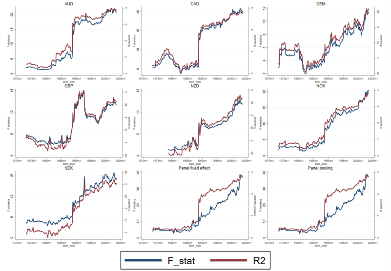
Figure B: F-statistic and R-squared of 20-year rolling window regressions
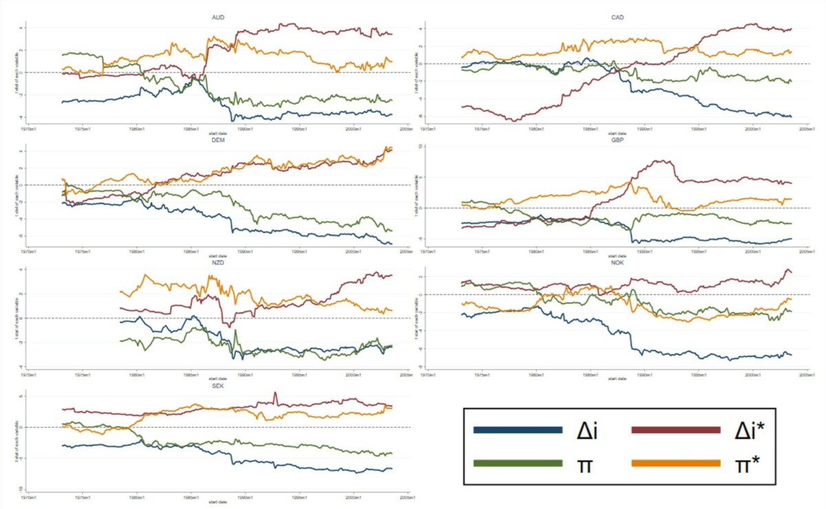
Figure C: t statistics of 20-year rolling window regressions
Monetary policy for the U.S. began to shift during the Volcker era, so that Taylor rules estimated on data beginning in the mid-1980s offer support for monetary stability. The advanced countries in our sample adopted inflation targeting a few years later: New Zealand in 1990, Canada in 1991, the U.K. in 1992, Sweden and Australia in 1993, Norway in 2001. One of the pillars of European Central Bank policy, beginning in 1999, is inflation targeting. Germany formally adopted inflation targeting in 1992 before the advent of the euro, though targeting inflation was always at the core of Bundesbank policy.
The paper produces further evidence to support the shift in monetary policy in these countries and its gradual increasing credibility. The important contribution here is that the success of the empirical model does not depend entirely on the risk and liquidity variables, which are important in tracking the movements of the dollar during times of global financial stress. The variables that represent the stance of monetary policy in the U.S. and the other countries are key to accounting for the good fit of the model today and its poor fit in the past. It is natural to attribute this change over time to the changing nature of monetary policy.
Empirical Exchange Rate Models are Better than You Think
Obviously, the fit of the model is not perfect. There may indeed be other factors driving exchange rates, including non-market “noise trading” that has been emphasized in some recent studies. However, it is likely that a major reason the fit is not perfect is because economists cannot perfectly measure the variables that theory says should drive the exchange rate: the stance of monetary policy, the level of global risk, the demand for liquidity, etc. Figure A certainly shows that the empirical model is able to capture major factors driving dollar exchange rates.
This post written by Charles Engel and Steve Pak Yeung Wu.